Custom Reporting and Analysis

Custom Reporting/Dashboards: Curated reports and dashboards to help clients make data-driven decisions and track key performance indicators (KPIs). Visualizations and Dashboards using Looker, Tableau, Excel, Kibana, Grafana, AWS, Jupyter/Jupyverse, Observable, Google Collab, Google Sheets, Dash, and others.
Data Visualization: Creating data visualizations to help clients understand their SEO performance and trends. Using tools like Matplotlib, Seaborn, Plotly, Dash, D3.js
Large Dataset Analysis: Analyzing massive datasets to uncover hidden trends, patterns, and insights that inform SEO strategies. There almost always isn’t a single point of failure when looking at SEO performance data and Technical SEO issues, but proper analysis and impact asssessment can help identify the most significant factors.
Machine Learning & NLP Actionable Insights: Applying machine learning and natural language processing (NLP) techniques to identify actionable insights from large datasets. Machine learning model output, NLP-based sentiment analysis report, and insights on user behavior and intent.
Voice Search and Conversational Analytics: Analyzing voice search data to identify conversational patterns, intent, and trends that inform SEO strategies.
Search Demand Models: Building predictive models to forecast search demand patterns, identifying trends, and informing SEO strategies.
Keyword Gap Analysis: Identifying gaps in keyword coverage to inform SEO strategies and optimize content.
Internal Link Analysis: Analyzing internal linking patterns to identify opportunities for improvement, optimize website structure, and enhance user experience.

e.g. Using networkx

import pandas as pd
import networkx as nx
import matplotlib.pyplot as plt
 
# Load the data
df = pd.read_csv('internal_links.csv')
 
# Create a directed graph
G = nx.from_pandas_edgelist(df, source='source', target='target', create_using=nx.DiGraph())
 
# Basic graph analysis
print("Number of nodes:", G.number_of_nodes())
print("Number of edges:", G.number_of_edges())
 
# Identify the most linked pages (in-degree)
in_degree = dict(G.in_degree())
sorted_in_degree = sorted(in_degree.items(), key=lambda x: x[1], reverse=True)
print("Most linked pages:", sorted_in_degree[:10])
 
# Identify the most linking pages (out-degree)
out_degree = dict(G.out_degree())
sorted_out_degree = sorted(out_degree.items(), key=lambda x: x[1], reverse=True)
print("Most linking pages:", sorted_out_degree[:10])
 
# Visualize the graph
plt.figure(figsize=(12, 8))
pos = nx.spring_layout(G, k=0.15)
nx.draw(G, pos, with_labels=False, node_size=50, node_color='blue', edge_color='gray')
plt.title('Internal Link Structure')
plt.show()

Log Files Analysis: Analyzing log files to track user behavior, identify trends, and inform SEO strategies.

e.g. using matplotlib

import pandas as pd
import matplotlib.pyplot as plt
import re
 
# Function to parse log file
def parse_log_line(line):
    pattern = r'(\S+) - - \[(.*?)\] "(\S+) (\S+) \S+" (\d+) (\d+)'
    match = re.match(pattern, line)
    if match:
        return match.groups()
    return None
 
# Read log file and parse each line
log_data = []
with open('access.log') as file:
    for line in file:
        parsed_line = parse_log_line(line)
        if parsed_line:
            log_data.append(parsed_line)
 
# Convert to DataFrame
columns = ['ip', 'timestamp', 'method', 'url', 'status', 'size']
df = pd.DataFrame(log_data, columns=columns)
 
# Convert timestamp to datetime
df['timestamp'] = pd.to_datetime(df['timestamp'], format='%d/%b/%Y:%H:%M:%S %z')
 
# Basic analysis
print("Total requests:", len(df))
print("Unique URLs:", df['url'].nunique())
print("Status code distribution:\n", df['status'].value_counts())
 
# Plotting the distribution of status codes
plt.figure(figsize=(10, 6))
df['status'].value_counts().sort_index().plot(kind='bar')
plt.xlabel('Status Code')
plt.ylabel('Number of Requests')
plt.title('Distribution of HTTP Status Codes')
plt.show()

SEO Forecasting: Using data-driven approaches to forecast future SEO trends, opportunities, and challenges. Forecasting via Facebook Prophet, Google’s Causal Impact tool, ARIMA (AutoRegressive Integrated Moving Average), and others

e.g. Facebook Prophet

from fbprophet import Prophet
import pandas as pd
 
# Load your data
df = pd.read_csv('your_seo_data.csv')
df['ds'] = pd.to_datetime(df['date'])
df['y'] = df['organic_traffic']
 
# Create and fit the model
model = Prophet()
model.fit(df)
 
# Make a future dataframe
future = model.make_future_dataframe(periods=365)
forecast = model.predict(future)
 
# Plot the forecast
fig = model.plot(forecast)

e.g. Google Causal Impact

from causalimpact import CausalImpact
import pandas as pd
 
# Load your data
data = pd.read_csv('your_seo_data.csv')
 
# Define pre and post intervention periods
pre_period = ['2020-01-01', '2020-06-30']
post_period = ['2020-07-01', '2020-12-31']
 
# Run Causal Impact analysis
ci = CausalImpact(data, pre_period, post_period)
print(ci.summary())
ci.plot()

e.g. ARIMA

import pandas as pd
import numpy as np
import matplotlib.pyplot as plt
from statsmodels.tsa.arima.model import ARIMA
 
# Load the data
df = pd.read_csv('seo_traffic.csv', parse_dates=['date'], index_col='date')
 
# Ensure the data is sorted by date
df = df.sort_index()
 
# Plot the data to visualize it
df['organic_traffic'].plot(figsize=(12, 6))
plt.title('Organic Traffic Over Time')
plt.xlabel('Date')
plt.ylabel('Organic Traffic')
plt.show()
 
# Define the model
model = ARIMA(df['organic_traffic'], order=(5, 1, 0))
 
# Fit the model
model_fit = model.fit()
 
# Print the model summary
print(model_fit.summary())
 
# Forecast the next 12 periods (e.g., months)
forecast_steps = 12
forecast = model_fit.forecast(steps=forecast_steps)
forecast_index = pd.date_range(start=df.index[-1], periods=forecast_steps + 1, closed='right')
 
# Create a DataFrame to hold the forecast
forecast_df = pd.DataFrame(forecast, index=forecast_index, columns=['Forecast'])
 
# Plot the original data and the forecast
plt.figure(figsize=(12, 6))
plt.plot(df['organic_traffic'], label='Historical Data')
plt.plot(forecast_df, label='Forecast', color='red')
plt.title('Organic Traffic Forecast')
plt.xlabel('Date')
plt.ylabel('Organic Traffic')
plt.legend()
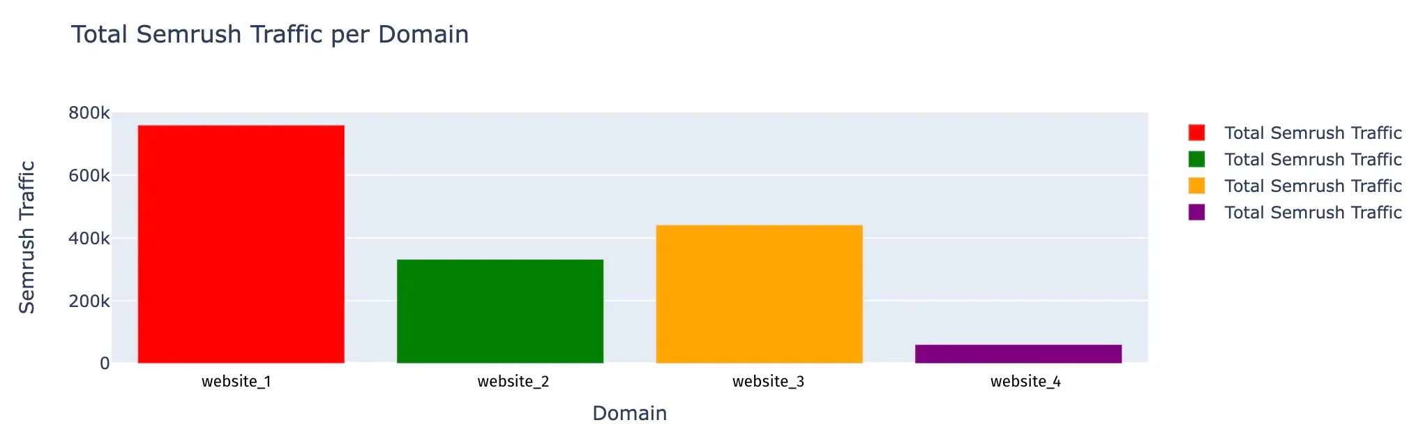
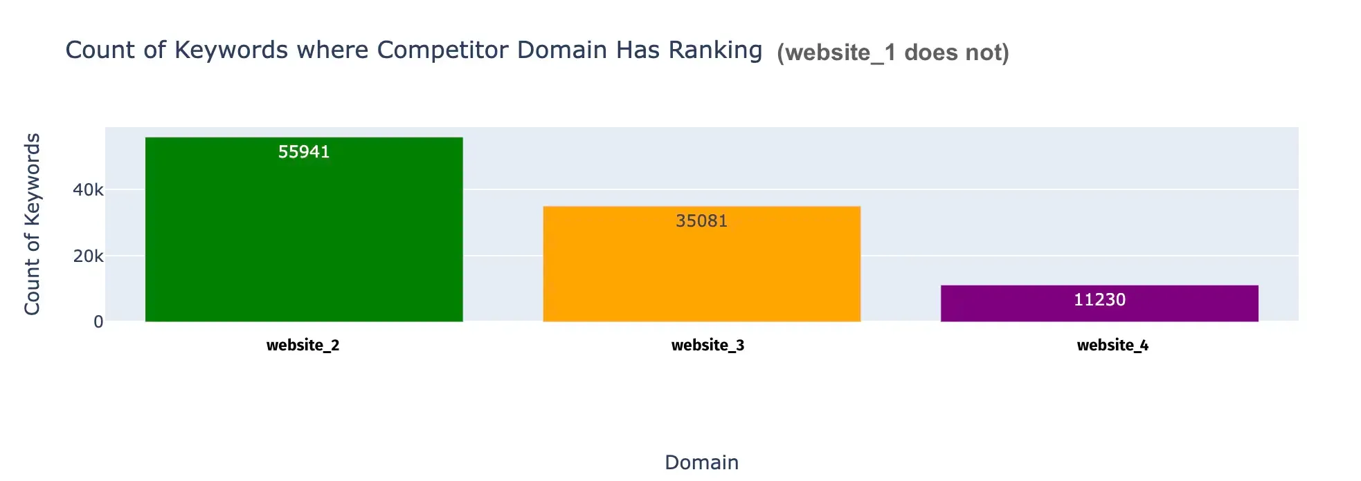
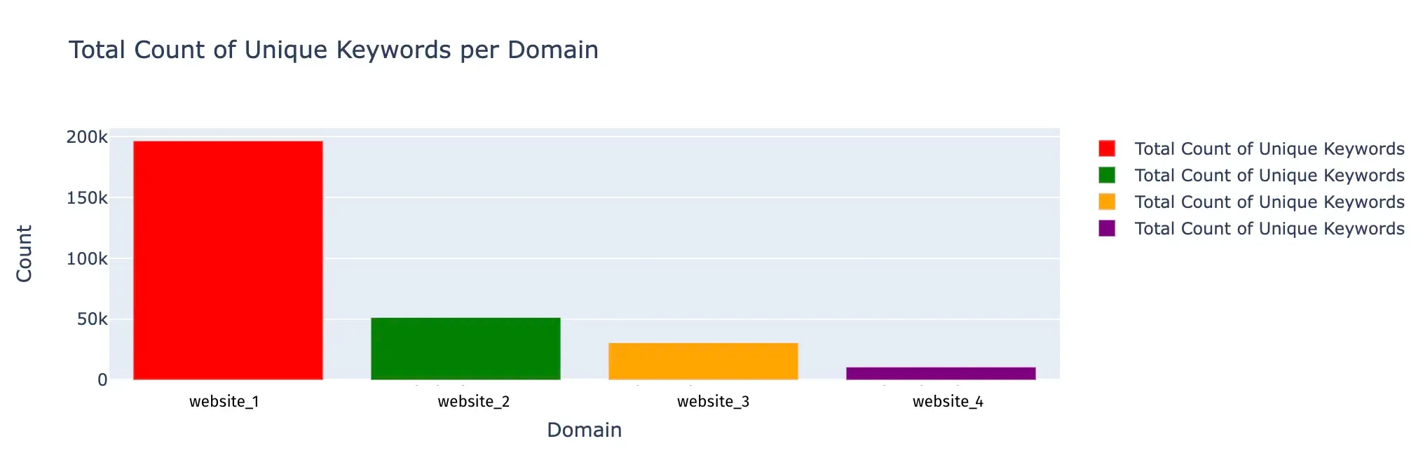
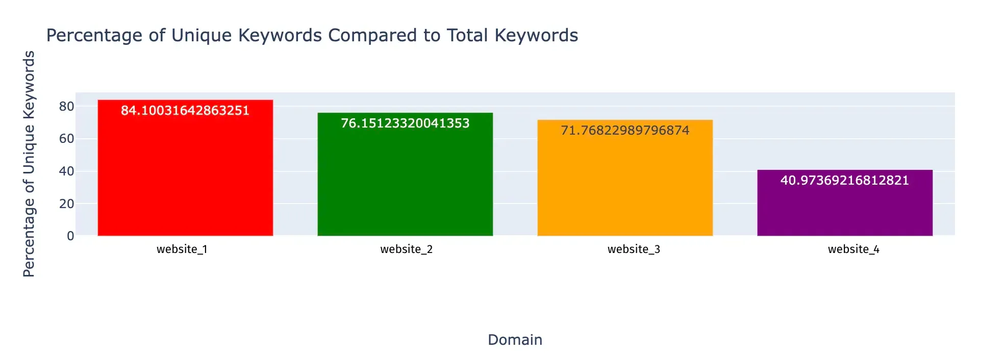
plt.show()

SEO TAM (Total Addressable Market): Identifying the total addressable market size for a specific keyword or topic, providing insights on competition and opportunity.

e.g. SEO_TAM_unique_competitor_rankings

e.g. SEO_TAM_count_unique_keywords

e.g. SEO_TAM_percentage_unique_keyword

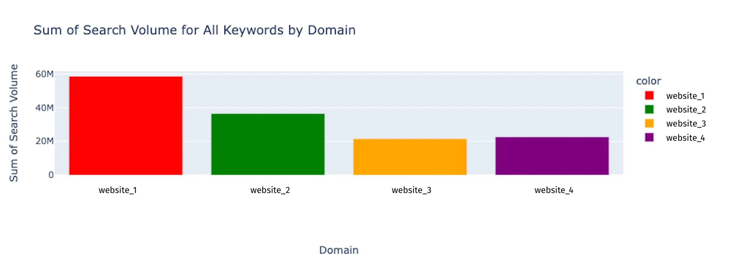
e.g. SEO_TAM_sum_search_volume_keywords

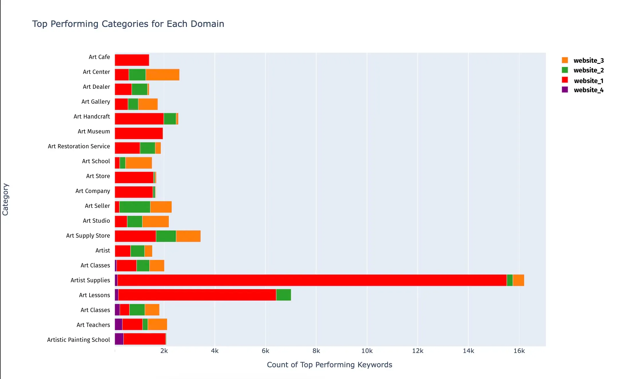
e.g. SEO_TAM_top_performing_categories

e.g. SEO_TAM_total_semrush_traffic